Customer Portal
Introduction
This guide provides an outline of steps required to set up to survey. Ideally, this document will be used along with the R2Sonic Operation Manual. The Operation Manual is always available in Sonic Control, under the Help Menu by selecting Help Topics. You can also request here. It is assumed that Sonic Control has been installed and communications have been established with the sonar and the Sonar Interface Module (SIM), as well as the auxiliary sensors (Sections 5.4 and 5.5 in the Operation Manual).
Offset Measurements (Section 2.9)
The data collection software requires extremely accurate offsets of the various sensors in order to calculate an accurate depth. To understand the acoustic center of the sonar, it is important to know how the sonar works. The projector transmits a single pulse, narrow alongtrack, and wide acrosstrack; the reference for the projector is the projector’s acoustic center. The acoustic pulse is reflected back to the receivers, and then the beams are formed; the receiver reference is the receiver’s acoustic center. The combination of the projector’s acoustic center and the receiver’s acoustic center becomes the acoustic center for the sonar and the point to measure with regards to the data collection software.
The acoustic center of the sonar, being a combination of the projector and receiver acoustic center, forms a point in space; in the horizontal plane, it is the position of the acoustic center of the projector. Where the data collection software requests an X and Y, or fore and starboard, enter the horizontal position of the projector’s acoustic center. The receiver determines the vertical measurement, so its acoustic center is used for the Z or vertical offset.
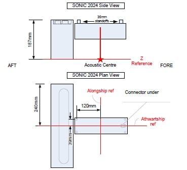
All measurements are in the manual, so they will not be repeated here; the above image is the concept of the acoustic center being a point in space.
The reference points for all other sensors require being measured and entered in the data collection software.
Patch Test (Appendix V)
When mounting the sonar head on a vessel, great care should be taken to ensure that the head is as perfectly aligned with the vessel axes as possible. Likewise, the motion sensor and heading sensor must also be installed as perfectly aligned as possible with the vessel axes. Even when great care is taken to align all sensors with the vessel axes, more accuracy is required, so a multibeam calibration (patch test) is carried out. Please refer to the Operation Manual Appendix V: The Patch Test for an in-depth description of the patch.
The patch test is used to determine the angular misalignment between the sonar head and the motion sensor, and the heading sensor. The values that are solved are the roll offset, the pitch offset, and the heading offset. Another test is performed to confirm that there is no system latency. Different bottom shapes are required; the roll test requires a flat bottom. All other tests require a feature or a steep slope. One data collection can often be used for two tests; using a channel slope, the flat channel area can be used for roll, and the side slope used for pitch, heading, and latency.
A bottom feature will work better for the pitch, heading, and latency data collections than a slope. The bottom feature can be a pipeline or a large wreck. Using a slope, the lines drawn to collect data should be perpendicular to the slope contours.
Key Points
- Collect sufficient data to have a statistically valid solution
- Perform all tests in as deep water as possible
- Roll test looks at outer beams
- Pitch and latency test looks at nadir data
- The heading test looks at overlapping data in the outer beams
- Good line steering is required
- Use lines for more than one test
- Take sound velocity casts
- Make sure of the data before leaving the patch test area
Sonar Settings (Section 5.6)
Frequency
R2Sonic multibeam echosounders can operate over a wide range of frequencies. When the frequency is changed, both the receive and transmit frequencies are changed. Usually, the highest frequency is used for the best acoustic resolution. However, as the survey goes into deeper water, the higher frequencies will be significantly affected by signal attenuation, so it is necessary to lower the frequency as the survey goes into deeper water.
Higher frequencies are absorbed more in a soft or muddy bottom over low frequencies. Therefore, lower frequencies will provide better swath coverage when used over a soft or muddy bottom.
Many times other acoustic devices will be used on a survey. To avoid interference with other acoustic sensors, the sonar can be tuned to a frequency that is away from the operating frequency of the other acoustic devices. Keep in mind that with acoustics, there are also what are called harmonics. A harmonic is a secondary (or tertiary) frequency at a multiple of the center operating frequency (or a fraction of the that frequency). A 200kHz single beam echosounder will have a harmonic at 400kHz, and this will be seen in the sonar as a radiating noise pattern. Tuning the sonar to 330kHz will eliminate the harmonic interference from the single beam echosounder.
Ping Rate Limit
The Ping Rate Limit is used to reduce the ping rate from the default value set by the Range setting. This setting is helpful when in shallow water. In shallow water, the Range will be short, and the ping rate will be high. Many times, when surveying in shallow water, the vessel slows down due to potential hazards. The high ping rate means much more data is being collected than is required; the ping rate limit is used to reduce the sonar ping rate from the high ping rate. If the Range setting is such that the ping rate is 30Hz that is 30 pings per second; use the ping rate limit to a value less than 30 to slow the ping rate and collect less unnecessary data.
If surveying in strong currents, the ping rate limit can help when going into the current because the current will slow the vessel. This will help keep the data concentration constant because surveying with the current will have the vessel moving much faster.
Bottom Sampling
There are multiple bottom sampling methods; the primary division is between Equiangle and Equidistant. Under both of those methods are the double and quad modes.
- Equiangle. All beams are at an equal angle. Because all beams are at the same angle, from the sonar head, there will be a concentration of beams within the nadir region, with the beams spreading out towards the outer swath.
- Equidistant. The beams are equally distributed across the swath. The sonar takes the nadir range and then computes the necessary beam angle to distribute the beams equally spaced across the swath. Equidistant mode assumes a more or less flat bottom and a swath angle of no more than 130°. Equidistant mode cannot be used when mapping vertical features. Equidistant mode should not be used with swath angles greater than 130°. With a wider swath, when the vessel rolls, the computation made to steer the beams equally across the swath will determine that the computation is no longer valid and will force the bottom sampling mode back to Equiangle.
- Double and Quad. The Double and Quad modes are enhancements to the Equiangle and Equidistant mode. The enhanced modes were developed for ROV surveys to provide better spatial coverage at the slow survey speed of an ROV. For surface vessels, the quad mode is also an enhancement over the standard modes. The double and quad mode do not add soundings; the mode provides a spatial distribution of soundings by juxtaposing the swath, left and right, on a ping to ping basis. In the below image, the normal Equidistant mode is seen as the soundings in line from the upper left corner; then, the system was changed to Equidistant quad halfway. The increased coverage created by the quad mode is easily seen.

- Ultra High Density (UHD). The one unique bottom sampling mode is Ultra High Density (UHD). UHD provides up to 1024 true and independent soundings per ping. UHD provides actual soundings, not interpolations or made up soundings. UHD is a proprietary process developed by R2Sonic.
Mission Mode
Unless the system is used in Forward Looking Sonar (FLS) mode, the two selections are Down, Bathy Normal, and Down, Bathy VFeature.
- Down, Bathy Normal. This mode is used for all surveying except when surveying a vertical surface or feature.
- Down, Bathy VFeature. The ‘V’ stands for Vertical; this mode is for mapping vertical features, such as quays, sheet piles, and pilings. Bathy, VFeature changes the bottom detection algorithm so that the sonar expects a magnitude detection in the outer beam (as opposed to a phase detection) and uses a smaller sampling period to avoid picking up extraneous data. Bathy VFeature has to be used with the Equiangle Bottom Sampling mode.
Sonar Operating Parameters (Section 5.16)
Tuning the sonar is done by adjusting three operating parameters: Power, Pulse Width, and Gain. Range is used to keep the ping timing sufficient so that all acoustic returns are received before the sonar pings again.
Range
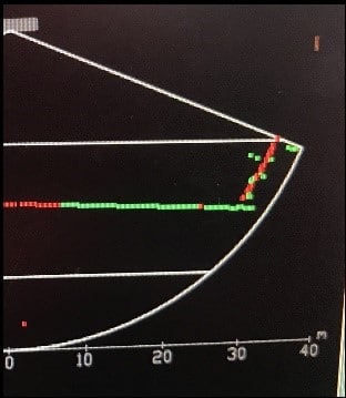
The Range setting sets the maximum slant range, which in turn sets the ping rate to allow all of the acoustic returns to be received before the sonar pings again. The correct Range setting can easily be determined by making sure all of the bottom detection dots in the wedge display are above the corners of the wedge.
If the Range is not set correctly, and the bottom detections are below the corner of the wedge, the receivers are cutoff before all the returning acoustic data is received; the last returns will be received in the next receive cycle. The acoustic data received in the wrong receive cycle will be seen as noise.
Power and Pulse Width
When the acoustic pulse is generated and transmitted into the water, the pulse is controlled by two factors. Power is the source level or amplitude of the pulse; the Pulse width is the length of time that pulse is transmitted into the water. Of course, another feature of the transmitted pulse is the frequency, which is discussed above.
The Power setting is in dB (decibels), which is logarithmic, not linear. The Power is increased in 3dB steps, which is a doubling in the source level output. When changing the Power settings, it must be kept in mind that each step up is doubling the output; each step down is cutting the source level in half.
Increasing the source level will have more influence within the nadir area of the swath. Be aware that when the Power is decreased it will not be reduced immediately because the capacitor banks used for the output power have to bleed down. Often the Power is decreased, and because it is not immediately seen in the acoustic display, the surveyor continues to lower the Power. When the capacitor bank does reach equilibrium, there may be insufficient source level being output. When reducing the Power, be patient. The TX Voltage in the Status window changes with a change in the Power setting; increasing and decreasing accordingly.
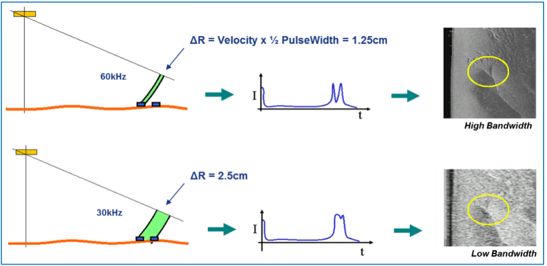
The Pulse Width setting determines how long the acoustic pulse is being transmitted. A shorter pulse width provides better acoustic resolution. A longer pulse width will help get more of the acoustic pulse to the outer areas of the swath. When surveying in soft sediment or muddy bottoms, increasing the Power will not aid the data as much as increasing the Pulse Width. Going into deeper water, the Pulse Width will have to be increased, possibly in significant steps.
The pulse width also determines the bandwidth.
- 15µsec – 30µsec = 60kHz bandwidth
- 35µsec – 65µsec = 30kHz bandwidth
Classic Range Resolution is defined as c*pw/2, where c is the speed of sound and pw is the pulse width. With a wider receiver bandwidth (factor 2 in the example), we can get 2 times better range resolution because this allows for a narrower pulse width (minimum pw is proportional to 1/BandWidth).
The Gain setting is very similar to a volume control. The Gain increases the sensitivity of the receivers. The general rule is to have sufficient acoustic Power going into the water to keep the receive gain low. If too much acoustic Power is being transmitted, then the receiver may be overdriven or saturated with the returning acoustic energy; when this happens, there will be artefacts in the data. Below, is discussed the Saturation Monitor, which is an aid in tuning the system.
Ocean Settings (Section 5.8)
All acoustic devices use Time Variable Gain (TVG). TVG is used because the first acoustic returns are the strongest and require the least amount of Gain. However, returns arriving later in the receive cycle are weaker and therefore require more Gain. TVG increases gain throughout the receive cycle. The two major factors that influence TVG are absorption and spreading loss.
Absorption
Absorption is frequency, salinity, and temperature dependent. The higher the frequency, the more warm and salty the water the more the absorption. Lower frequencies, fresher water, and cooler water will have the least amount of absorption. A built-in calculator calculates the correct absorption value based on the frequency, salinity, and water temperature.
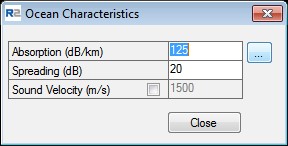
Spreading Loss
Spreading loss is the loss of intensity of a sound wave, due to the dispersion of the wavefront. It is a geometrical phenomenon and is independent of frequency, temperature, or salinity. The default value is 20dB. Spreading Loss should be increased when surveying into deeper water. The default of 20dB is good for about 30 meters depth, and should be increased if the survey continues into deeper water.
Saturation Monitor (Section 5.10.2)
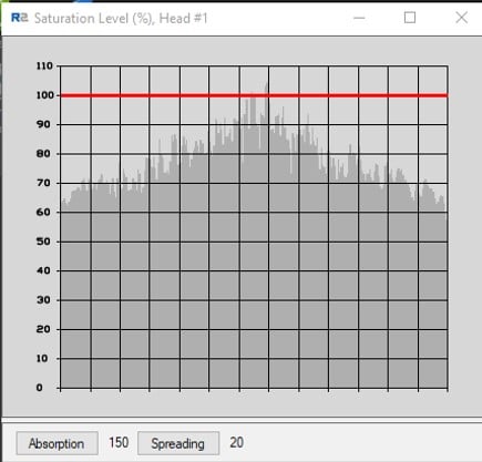
The Saturation Monitor is found under the Status menu. The Saturation Monitor was initially created as a visual aid for backscatter surveys, where it is critical that the receivers remain out of saturation. The display shows the intensity level (in percentage) as seen in the receivers.
After introducing the Saturation Monitor, it became evident that it was also an excellent tool to use for bathymetry surveys. The Saturation Monitor immediately shows the effect of changes in Power, Pulse Width, Gain, Absorption, and Spreading Loss. Before the Saturation Monitor, it was possible to use too much Power or too much Gain without the user realizing they had over-driven the receivers. There would be noticeable artefacts in data like a nadir track.
The red line signifies 100% saturation; the user should adjust the sonar to keep the intensities below the red line. Ideally, a range of 60% to 80% should be maintained for the best data.
Because the outer beam data will be slightly weaker while the nadir data will be stronger, the shape of the intensities will not be even across.
The buttons to adjust the Absorption and Spreading Loss are for backscatter survey use. However, this does not mean that the settings cannot be adjusted for a bathymetry survey when it is warrantied.
Troubleshooting
- The head and SIM can be discovered, but no data in the display –Check that the computer’s IP is the same as the IP for the GUI in network settings; default is 10.0.1.102
- Only the SIM can be discovered – Check that Sonar Power is checked on in Sonar Settings. Check the seating of decklead to receiver
- In the Saturation Monitor, the intensities are very low, and data quality is poor – Open System Status and check that the TX Voltage increases with an increase in the Power setting.
- The GUI seems sluggish; things just do not seem some ‘right’ – Start with making sure that Sonic Control is installed in its own folder on the hard drive’s root directory. In Sonic Control, go to File – Load Settings and browse for the Default Settings folder; load the default settings for the configuration being used. Loading the default settings will reset the GUI to factory defaults; Discover and Apply have to be done again, as well as all sensor interfacing parameters have to be set up.